Tutorial 2

This is a tutorial for developing a linear regressor using keras. This tutorial takes after Tutorial 1 which can be found in the ML4Art page.

Overview

Our motive in this tutorial is to create a linear regressor using keras. We will implement a neural network which will attempt to learn a particular function we provide it. It will be a 3 dimensional function and therefore has two inputs (which will be the x and y co-ordinates). The value to be predicted will be the z co-ordinate.

Creating our training data

Since we are trying to model our own function, there is no pre existing database which we wish to use. Thus, let us create our training data which contains 200 random x and 200 random y values.

np.random.seed(seed = 99)
X = np.random.uniform(-1, 1, size=100)
Y = np.random.uniform(-1, 1, size=100)

The np.random.seed() function sets the random seed so that every time we execute the program, the same data values are generated.

The function we wish to model is: z = sin(x^2 + y^2 - 1)

Thus, we write the following piece of code:

R = 1*(X**2) + 2*(Y**2) - 1
Z = np.sin(R)

Constructing our Neural Network

We already went about creating a neural network in our previous tutorial. We do exactly the same thing here:

input_img = Input(shape=(2,))

encoded = Dense(32, activation='sigmoid')(input_img)

encoded = Dense(16, activation='sigmoid')(encoded)
encoded = Dense(8, activation='sigmoid')(encoded)
encoded = Dense(4, activation='sigmoid')(encoded)

encoded = Dense(2, activation='sigmoid')(encoded)
decoded = Dense(1, activation='linear')(encoded)
autoencoder = Model(input_img, decoded)

autoencoder.compile(optimizer='adadelta', loss='binary_crossentropy')

The funnel architecture (as we would like to call it) has been found to offer the same benefits of the slab architecture (two layers of 1000 nodes) with far lower number of computations. Hence, we follow the funnel architecture here.

We now fit our training data:

X_train = [[X[i],Y[i]] for i in range(len(X))]
y_train = Z
autoencoder.fit(X_train, y_train,
                epochs=50)

We have literally zipped the X and Y arrays so that we can provide two inputs and obtain 1 output.

Building our testing data

We will now construct our testing data that comprises of 1000x1000 points. We are doing something unconventional where the number of testing points are far greater than the number of the training points. This is solely done to study the learning behavior of the network.

We will first construct a numpy array that has 1000 points and then take the cross product of that array with itself. Once we have done so, we will extract all the x and y co-ordinates into two distinct arrays.

A = np.arange(-1, 1, 0.002)
inter = [(x, y) for x in A for y in A]

A = [x[0] for x in inter]
B = [x[1] for x in inter]
A = np.array(A)
B = np.array(B)

Now that our X and Y values are stored in A and B respectively, we will construct a new zipped version of our test data so that we may feed it into our network. This could've been done before also (instead of constructing an array of tuples as inter).

test = [[A[i],B[i]] for i in range(len(A))]
decoded_imgs = autoencoder.predict(test)

Plotting a graph

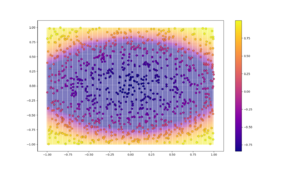
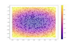
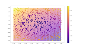
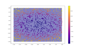
Now that we have our training and test data, we plot the testing data in the background and the test data as bigger points in the foreground. By doing so, just at the glance of a pair of eyes, we will know how well the regressor has done and whether the predictions agree with the ground truth.

plt.scatter(A, B, c=decoded_imgs, cmap='plasma', s=0.01)
plt.scatter(X, Y, c=Z, cmap='plasma', s=50,edgecolor='black', linewidth='0.25')

plt.colorbar()
plt.show()

The first three arguments to the scatter function are the X, Y and Z co-ordinates. cmap represents the color map scheme and the s parameter is for the size of points. Other attributes are self explanatory.

Sample Images

Here are a few sample images:

A contour plot for training:

The predicted model by a simple NN: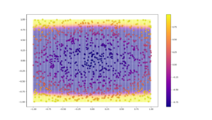

Predicted model by a deep multilevel NN:

A deep NN with all layers as sigmoid:

A deep NN with the last layer as ReLU: