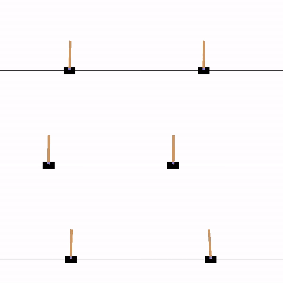
CartPole DQN

Overview

This tutorial will show you how to solve the popular CartPole problem using deep Q-learning. The CartPole problem is as follows:

A pole is attached by an un-actuated joint to a cart, which moves along a frictionless track.
The system is controlled by applying a force of +1 or -1 to the cart.
The pendulum starts upright, and the goal is to prevent it from falling over.
A reward of +1 is provided for every timestep that the pole remains upright.
The episode ends when the pole is more than 15 degrees from vertical,
or the cart moves more than 2.4 units from the center.

Tutorial

This section will walk you through the steps of solving the CartPole problem with a deep Q-network. This tutorial is written for python 3.

Packages

You must first pip install the following packages: gym keras and numpy

DQN Agent

The first step of our implementation will be creating a DQNAgent object. This object will manage the state of our learning, and is independent of the CartPole problem. It has all the generic parts of a Q-learning agent and can be reused for other deep Q-learning applications.

Imports

Start by creating a file DQNAgent.py and include the following imports:

from keras.layers import Input, Dense
from keras.optimizers import RMSprop
from keras.models import Model
from collections import deque

Constructor

The reason for each import will become apparent as our implementation continues. Next add a blank DQNAgent class with an empty constructor.

class DQNAgent:
    
    def __init__(self):
        pass

This class will take in all of our hyperparemeters, so let's update our constructor to take in those parameters. We also provide some default values for some of those hyperparameters.

class DQNAgent:
    
    def __init__(self, input_dim, output_dim, learning_rate=.005,
            mem_size=5000, batch_size=64, gamma=.99, decay_rate=.0005):
        pass

• input_dim is the number of input nodes for our DQN.
• output_dim is the number of output nodes for our DQN.
• learning_rate is a Keras parameter for our network describing how much we value new information.
• mem_size is the maximum number of instances allowed in our bucket for experience replay.
• batch_size is the number of experience tuples we train our model on each replay event.
• gamma is our discount factor for the Bellman equation update.
• decay_rate is the rate at which exploration probability decays.

Now for the next step, we complete our constructor by saving all of these parameters as instance variables, defining a neural network model, and defining a few other parameters.

def __init__(self, input_dim, output_dim, learning_rate=.005,
        mem_size=5000, batch_size=64, gamma=.99, decay_rate=.0005):

    # Save instance variables.
    self.learning_rate = learning_rate
    self.batch_size = batch_size
    self.gamma = gamma
    self.decay_rate = decay_rate

    # Define other instance variables.
    self.explore_p = 1 # The current probability of taking a random action.
    self.memory = deque(maxlen=mem_size) # Define our experience replay bucket as a deque with size mem_size.

    # Define and compile our DQN. This network has 3 layers of 24 nodes. This is sufficient to solve
    # CartPole, but you should definitely tweak the architecture for other implementations.
    input_layer = Input(shape=(input_dim,))
    hl = Dense(24, activation="relu")(input_layer)
    hl = Dense(24, activation="relu")(hl)
    hl = Dense(24, activation="relu")(hl)
    output_layer = Dense(output_dim, activation="linear")(hl)
    self.model = Model(input_layer, output_layer)
    self.model.compile(loss="mse", optimizer=RMSprop(lr=learning_rate))

Act

The most fundamental part of a Q-learning problem is the ability for the agent to take an action. Actions are either determined by the current policy (based off Q-function values) or are picked randomly, depending on the current exploration probability. We now define an act function which, given the current state of the environment, determines which action to take next. Note that with OpenAI gym, actions correspond to integers (0, 1, 2, ...).

def act(self, state):
    # First, decay our explore probability
    self.explore_p *= 1 - self.decay_rate
    # With probability explore_p, randomly pick an action
    if self.explore_p > np.random.rand():
        return np.random.randint(self.output_dim)
    # Otherwise, find the action that should maximize future rewards according to our current Q-function policy.
    else:
        return np.argmax(self.model.predict(np.array([state]))[0])