MC1-Project-2

Overview

In this project you will use what you learned about optimizers to optimize a portfolio. That means that you will find how much of a portfolio's funds should be allocated to each stock so as to optimize it's performance. In this case we define "optimal" as maximum Sharpe ratio.

You will leverage the functions you created in the last project that assessed the value of a portfolio with a given set of allocations.

An older version of this project: MC1-Project-2-archive

Task

Implement a Python function named optimize_portfolio() in the file optimization.py that can find the optimal allocations for a given set of stocks. You should optimize for Sharpe ratio.

The function should accept as input a list of symbols as well as start and end dates and return a list of floats (as a one-dimensional numpy array) that represents the allocations to each of the equities. You should take advantage of routines developed in the portfolio analysis project to compute daily portfolio value and statistics.

You are given the following inputs for optimizing a portfolio:

• A date range to select the historical data to use (specified by a start and end date)
• Symbols for equities (e.g., GOOG, AAPL, GLD, XOM). Note: You should support any symbol in the data directory.

Your goal is to find allocations to the symbols that maximizes Sharpe Ratio. Assume 252 trading days in a year and a risk free rate of 0.0. You should implement the following API EXACTLY, if you do not your submission will be penalized at least 20%.

import datetime as dt
allocs = \
    optimize_portfolio(sd=dt.datetime(2008,1,1), ed=dt.datetime(2009,1,1), \
    syms=['GOOG','AAPL','GLD','XOM'], gen_plot=False)

Where the returned output is:

• allocs: A 1-d Numpy array of allocations to the stocks, must sum to 1.0

The input parameters are:

• sd: A datetime object that represents the start date
• ed: A datetime object that represents the end date
• syms: A list of symbols that make up the portfolio (note that your code should support any symbol in the data directory)
• gen_plot: If True, create a plot named plot.png

ALL of your code should be present in the single file optimization.py

Template

Instructions:

• Download mc1_p2.zip, unzip inside ml4t/
• Copy analysis.py (your solution for MC1-Project-1) to mc1_p2/portfolio/.
• Implement the find_optimal_allocations() function in mc1_p2/portfolio/optimization.py.
• To execute, run python -m portfolio.optimization from mc1_p2/ directory.

Your solution to the optimization problem should leverage the software you developed in the last assignment. to test your code, we will be calling optimize_portfolio(). Make sure the output and plot look like the examples shown below.

Suggestions

Refer to comments in the provided helper code for pointers regarding how to implement it. In order to specify bounds and constraints when using the scipy.optmize module, you'll need to use a special syntax explained here: http://docs.scipy.org/doc/scipy/reference/generated/scipy.optimize.minimize.html

For bounds, you simply need to pass in a sequence of 2-tuples (<low>, <high>). Just remember that you need to supply as many tuples as the number of stocks in your portfolio.

For constraints, it's a little tricky. You need to pass in a sequence of dicts (dictionaries), one dictionary per constraint. Each dictionary must specify the type of constraint ('eq' for equality, or 'ineq' for inequality), and a function that returns 0 only when the input satisfies the constraint (this is the same input that is supplied to your evaluation function). E.g. to constrain the sum of all values in the input array to be less than 50, you could pass in the following (lambdas are just anonymous functions defined on-the-spot):

constraints = ({ 'type': 'eq', 'fun': lambda inputs: 50.0 - np.sum(inputs) })

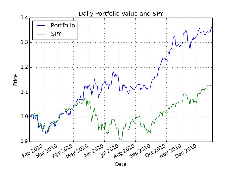
Example output 1

Here's an example output for your function. These are actual correct values that you can use to check your work.

Start Date: 2010-01-01
End Date: 2010-12-31
Symbols: ['GOOG', 'AAPL', 'GLD', 'XOM']
Optimal allocations: [  5.38105153e-16   3.96661695e-01   6.03338305e-01  -5.42000166e-17]
Sharpe Ratio: 2.00401501102
Volatility (stdev of daily returns): 0.0101163831312
Average Daily Return: 0.00127710312803
Cumulative Return: 0.360090826885

Corresponding comparison plot:

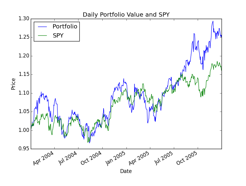
Example output 2

Start Date: 2004-01-01
End Date: 2006-01-01
Symbols: ['AXP', 'HPQ', 'IBM', 'HNZ']
Optimal allocations: [  7.75113042e-01   2.24886958e-01  -1.18394877e-16  -7.75204553e-17]
Sharpe Ratio: 0.842697383626
Volatility (stdev of daily returns): 0.0093236393828
Average Daily Return: 0.000494944887734
Cumulative Return: 0.255021425162

Example output 3

Start Date: 2004-12-01
End Date: 2006-05-31
Symbols: ['YHOO', 'XOM', 'GLD', 'HNZ']
Optimal allocations: [ -3.84053467e-17   7.52817663e-02   5.85249656e-01   3.39468578e-01]
Sharpe Ratio: 1.5178365773
Volatility (stdev of daily returns): 0.00797126844855
Average Daily Return: 0.000762170576913
Cumulative Return: 0.315973959221

Example output 4

Start Date: 2005-12-01
End Date: 2006-05-31
Symbols: ['YHOO', 'HPQ', 'GLD', 'HNZ']
Optimal allocations: [ -1.67414005e-15   1.01227499e-01   2.46926722e-01   6.51845779e-01]
Sharpe Ratio: 3.2334265871
Volatility (stdev of daily returns): 0.00842416845541
Average Daily Return: 0.00171589132005
Cumulative Return: 0.229471589743

Minor differences in float values may arise due to different implementations.

What to turn in

Be sure to follow these instructions exactly!

Via T-Square, submit as attachments (no zip files; refer to schedule for deadline):

• Your code as optimization.py (only the function optimize_portfolio() will be tested). Make sure that all necessary code is in that file.
• Plot comparing the optimal portfolio with SPY as comparison_optimal.png using the following parameters:
  Start Date: 2010-01-01, End Date: 2010-12-31, Symbols: ['GOOG', 'AAPL', 'GLD', 'HNZ']

Unlimited resubmissions are allowed up to the deadline for the project.

Rubric

• Part 1: Chart is correct [20 points]
  • Normalized values start at 1.0 on left (10 points)
  • Shape of curves are correct (10 points)
• Part 2: 10 test cases [80 points]
  We will test your code against 10 cases (8 points per case). Each case will be deemed "correct" if:
  • sum(allocations) = 1.0 +- 0.02
  • Each allocation is between 0 and 1.0 +- 0.02 (negative allocations are allowed if they are very small)
  • Each allocation matches reference solution +- 0.10

Required, Allowed & Prohibited

Required:

• Your project must be coded in Python 2.7.x.
• Your code must run on one of the university-provided computers (e.g. buffet02.cc.gatech.edu), or on one of the provided virtual images.
• Your code must run in less than 5 seconds on one of the university-provided computers.

Allowed:

• You can develop your code on your personal machine, but it must also run successfully on one of the university provided machines or virtual images.
• Your code may use standard Python libraries.
• You may use the NumPy, SciPy and Pandas libraries. Be sure you are using the correct versions.
• You may reuse sections of code (up to 5 lines) that you collected from other students or the internet.
• Code provided by the instructor, or allowed by the instructor to be shared.

Prohibited:

• Any libraries not listed in the "allowed" section above.
• Any code you did not write yourself (except for the 5 line rule in the "allowed" section).
• Any Classes (other than Random) that create their own instance variables for later use (e.g., learners like kdtree).
• Camels and other dromedaries.