Difference between revisions of "MC1-Project-1"
| Line 57: | Line 57: | ||
* Your job is to implement these functions, with exactly the APIs (inputs and outputs) described below. DO NOT modify the list of input parameters or output results because they will be tested by the auto grading system: | * Your job is to implement these functions, with exactly the APIs (inputs and outputs) described below. DO NOT modify the list of input parameters or output results because they will be tested by the auto grading system: | ||
| − | * <tt>'''get_portfolio_value'''(prices, allocs, start_val)</tt>: Compute daily portfolio value given stock prices, allocations and starting value.<br />Ensure that it returns a pandas <tt>Series</tt> or <tt>DataFrame</tt> (with a single column). | + | ** <tt>'''get_portfolio_value'''(prices, allocs, start_val)</tt>: Compute daily portfolio value given stock prices, allocations and starting value.<br />Ensure that it returns a pandas <tt>Series</tt> or <tt>DataFrame</tt> (with a single column). |
| − | * <tt>'''get_portfolio_stats'''(port_val, daily_rf, samples_per_year)</tt>: Calculate statistics on daily portfolio value, given daily risk-free rate and data sampling frequency.<br />This function should return a ''tuple'' consisting of the following statistics (in order): cumulative return, average daily return, standard deviation of daily return, Sharpe ratio<br />Note: The return statement provided ensures this order. | + | ** <tt>'''get_portfolio_stats'''(port_val, daily_rf, samples_per_year)</tt>: Calculate statistics on daily portfolio value, given daily risk-free rate and data sampling frequency.<br />This function should return a ''tuple'' consisting of the following statistics (in order): cumulative return, average daily return, standard deviation of daily return, Sharpe ratio<br />Note: The return statement provided ensures this order. |
| − | * <tt>'''plot_normalized_data'''(df, title, xlabel, ylabel)</tt>: Normalize given stock prices and plot for comparison.<br />This is used to create a chart that illustrates the value of your portfolio over the year and compares it to SPY.<br />Note: Before plotting, portfolio and SPY values should be normalized to 1.0 at the beginning of the period. Also, use the <tt>plot_data()</tt> utility function to generate and show your plot. | + | ** <tt>'''plot_normalized_data'''(df, title, xlabel, ylabel)</tt>: Normalize given stock prices and plot for comparison.<br />This is used to create a chart that illustrates the value of your portfolio over the year and compares it to SPY.<br />Note: Before plotting, portfolio and SPY values should be normalized to 1.0 at the beginning of the period. Also, use the <tt>plot_data()</tt> utility function to generate and show your plot. |
* Refer to each function's documentation (in triple quotes after the <tt>def</tt> line) for details about the parameters and expected return values. | * Refer to each function's documentation (in triple quotes after the <tt>def</tt> line) for details about the parameters and expected return values. | ||
* Implement each function; feel free to modify <tt>test_run()</tt> and <tt>assess_portfolio()</tt> to write additional tests (e.g. to call and inspect the functions individually). | * Implement each function; feel free to modify <tt>test_run()</tt> and <tt>assess_portfolio()</tt> to write additional tests (e.g. to call and inspect the functions individually). | ||
Revision as of 00:00, 18 September 2015
Contents
Overview
A portfolio is a collection of stocks (or other investment options) and corresponding allocations of money to each of them. In order to evaluate and compare different portfolios, we first need to compute certain metrics, based on available historical data.
The primary goal of this assignment is to introduce you to this form of portfolio analysis. You will use pandas for reading in data, calculating various statistics and plotting a comparison graph.
Task
You are given the following inputs for analyzing a portfolio:
- A date range to select the historical data to use (specified by a start and end date)
- Symbols for equities (e.g., GOOG, AAPL, GLD, XOM)
- Allocations to the equities at the beginning of the simulation (e.g., 0.2, 0.3, 0.4, 0.1)
- Total starting value of the portfolio (e.g. $1,000,000)
Your goal is to compute the daily portfolio value over given date range, and then the following statistics for the overall portfolio:
- Cumulative return
- Average daily return
- Standard deviation of daily returns
- Sharpe ratio of the overall portfolio, given daily risk free rate (usually 0), and yearly sampling frequency (usually 252, the no. of trading days in a year)
Note: Assume the risk free rate is zero.
Template
A template is provided for you to get started with the project: mc1_p1.zip
Download and unzip it inside ml4t/. It should consist of:
- mc1_p1/: Root directory for the template
- portfolio/: Python package with all project-specific code
- analysis.py: Main project script with functions you need to implement, as well as test code
- output/: Directory to store all program outputs, including plots
- util.py: Utility functions (do not modify these, unless instructed)
- portfolio/: Python package with all project-specific code
Notes:
- Ignore any file named __init__.py; they are used to mark directories as Python packages.
- We assume your data/ directory is one level up, (i.e., ../data/). That directory should contain all stock data, in CSV files (e.g. GOOG.csv, AAPL.csv, etc.)
- To execute the main script, make sure your current working directory is mc1_p1/, then run:
python -m portfolio.analysis
This directory structure may seem a little complicated at first, but it will help you organize your code better.
Instructions
- Open: portfolio/analysis.py
Function documentation and code comments should help you understand what you need to do. If it is still not clear, read the detailed instructions below. - Look at the function: test_run()
Here we have set up some sample inputs, which are then passed to the assess_portfolio() function:
start_date = '2010-01-01'
end_date = '2010-12-31'
symbols = ['GOOG', 'AAPL', 'GLD', 'XOM']
allocs = [0.2, 0.3, 0.4, 0.1]
start_val = 1000000
assess_portfolio(start_date, end_date, symbols, allocs, start_val)
- Now look at: assess_portfolio()
It first reads historical data for the given date range and symbols, and then uses three helper functions to simulate and assess the performance of the stock portfolio. assess_portfolio() is a helper function that is used to exercise your code. It will not be evaluated in the grading process.
- Your job is to implement these functions, with exactly the APIs (inputs and outputs) described below. DO NOT modify the list of input parameters or output results because they will be tested by the auto grading system:
- get_portfolio_value(prices, allocs, start_val): Compute daily portfolio value given stock prices, allocations and starting value.
Ensure that it returns a pandas Series or DataFrame (with a single column). - get_portfolio_stats(port_val, daily_rf, samples_per_year): Calculate statistics on daily portfolio value, given daily risk-free rate and data sampling frequency.
This function should return a tuple consisting of the following statistics (in order): cumulative return, average daily return, standard deviation of daily return, Sharpe ratio
Note: The return statement provided ensures this order. - plot_normalized_data(df, title, xlabel, ylabel): Normalize given stock prices and plot for comparison.
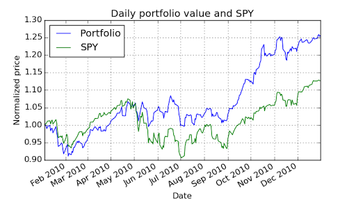
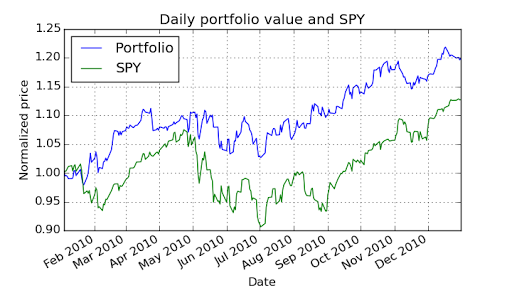
This is used to create a chart that illustrates the value of your portfolio over the year and compares it to SPY.
Note: Before plotting, portfolio and SPY values should be normalized to 1.0 at the beginning of the period. Also, use the plot_data() utility function to generate and show your plot.
- get_portfolio_value(prices, allocs, start_val): Compute daily portfolio value given stock prices, allocations and starting value.
- Refer to each function's documentation (in triple quotes after the def line) for details about the parameters and expected return values.
- Implement each function; feel free to modify test_run() and assess_portfolio() to write additional tests (e.g. to call and inspect the functions individually).
- Save the comparison plot as comparison.png (you should be able to do this directly from the plot window).
- Submit your final analysis.py along with comparison.png once you are confident that your functions are working as expected.
Note: In order to avoid issues with grading, make sure your functions accept exactly the parameters and return the value(s) that are defined in the respective function documentation. Also, turn off all printing and plotting from within these functions, unless instructed (e.g. plot_normalized_data() should generate a plot).
Suggestions
Here is a suggested high-level outline for what your script needs to do:
- Read in adjusted closing prices for the 4 equities.
- Normalize the prices according to the first day. The first row for each stock should have a value of 1.0 at this point.
- Multiply each column by the allocation to the corresponding equity.
- Multiply these normalized allocations by starting value of overall portfolio, to get position values.
- Sum each row (i.e. all position values for each day). That is your daily portfolio value.
- Compute statistics from the total portfolio value.
Here are some notes and assumptions:
- When we compute statistics on the portfolio value, we do not include the first day.
- We assume you are using the data provided. If you use other data your results may turn out different from ours. Yahoo's online data changes every day. We could not build a consistent "correct" answer based on "live" Yahoo data.
- Assume 252 trading days/year.
Make sure your assess_portfolio() function gives correct output. Check it against the examples below.
Example output
These are actual correct examples that you can use to check your work.
Example 1
Start Date: 2010-01-01
End Date: 2010-12-31
Symbols: ['GOOG', 'AAPL', 'GLD', 'XOM']
Allocations: [0.2, 0.3, 0.4, 0.1]
Sharpe Ratio: 1.51819243641
Volatility (stdev of daily returns): 0.0100104028
Average Daily Return: 0.000957366234238
Cumulative Return: 0.255646784534
Example 2
Start Date: 2010-01-01
End Date: 2010-12-31
Symbols: ['AXP', 'HPQ', 'IBM', 'HNZ']
Allocations: [0.0, 0.0, 0.0, 1.0]
Sharpe Ratio: 1.30798398744
Volatility (stdev of daily returns): 0.00926153128768
Average Daily Return: 0.000763106152672
Cumulative Return: 0.198105963655
Example 3
Start Date: 2010-06-01
End Date: 2010-12-31
Symbols: ['GOOG', 'AAPL', 'GLD', 'XOM']
Allocations: [0.2, 0.3, 0.4, 0.1]
Sharpe Ratio: 2.21259766672
Volatility (stdev of daily returns): 0.00929734619707
Average Daily Return: 0.00129586924366
Cumulative Return: 0.205113938792
What to turn in
Be sure to follow these instructions diligently!
Submit via T-Square as attachments only (no zip files please):
- Your code as analysis.py (please use this EXACT filename)
- Your plot of daily portfolio value versus SPY as comparison.png (use EXACT filename)
The plot should be generated using the following:, Start Date: 2010-01-01, End Date: 2010-12-31, Symbols: ['GOOG', 'AAPL', 'GLD', 'XOM'], Allocations: [0.2, 0.2, 0.4, 0.2]
Unlimited resubmissions are allowed up to the deadline for the project.

